Is a ConvNet-based model always the best solution?
With all the achievements of ConvNet-based models in computer vision, such as accurate classification and localization of a variety of different objects of varying size and view angles, one might forget about non-learning based computer vision techniques. I think a strict focus on ConvNets is a mistake and in this post I will illustrate why.
The strengths of ConvNet-based models for say object classification is its robustness against changes such as in illumination or angle. However, training a ConvNet generally requires a large amount of labelled data, and acquiring these labels can be tedious and time consuming. On the other hand, a non-learning based approach requires you to tune the parameters. Table 1 provides an overview of selected criteria. If you want to learn more about the details of learned approaches see our section here.
| Criteria | ConvNet-based | Non-learning based |
|---|---|---|
| Robustness | high | low |
| Transparency | low | high |
| Effort to set up | high | low |
| Running time | high | low |
Table 1: Strengths and weaknesses of learning and non-learning based techniques.
Now which approach is better? It depends on the problem you are looking to solve. Generally, I think the first question to answer is if the problem domain is relatively static. If for example you expect images taken from a variety of angles and different cameras, then a learned approach might be better. In the following example, I will illustrate this.
Case study: Lane line detection
Recently, I’ve been working on our object detector, which detects vehicles, pedestrians and more objects in traffic. I wanted to add lane line detection and found that most examples use a pipeline similar to what is shown in figure 1, see here and here.

Basically, it takes the input image, removes the colour channels and detects edges using Canny Edge Detection. Then, a triangularly shaped region of interest is cropped out where we expect the lanes to lie. In this region of interest, we apply the Hough transform which finds edges along the lane lines. We then use these edges to fit two linear functions along it, one on the left and one on the right, which become our detected lane lines.
In this pipeline you might notice two things. Firstly, it uses components which are problem-specific. For example, by selecting the region of interest, we focus on a specific part of the image where we expect the lane lines to be. Additionally, the Hough transform, as it is used here, is able to detect straight lines only. Consequently, we commit to certain conditions we expect the problem to meet in order to work by the selection of the data pipeline.
Secondly, the difficulty here is to get the parameters right. You do this by taking some example images and tune one parameter at a time. While this is time consuming, I argue that labelling hundreds of images is even more tedious.
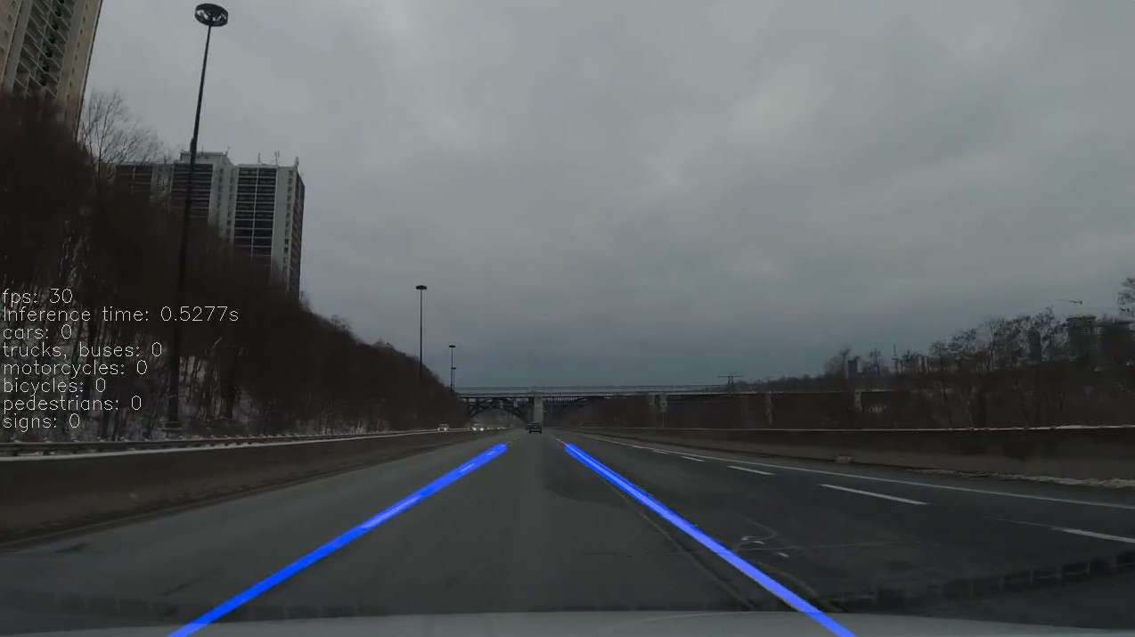
After some experimenting I came up with the lines shown in figure 2.

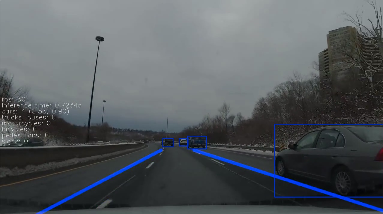
This looks great so far which is no surprise since it is exactly what I tuned the model for. In figure 3, the road curves slightly which leads to some occasional issue. This is no surprise either because in the selection of the pipeline, we specified that we detect straight lines. So the curvier the road, the poorer the model will work.

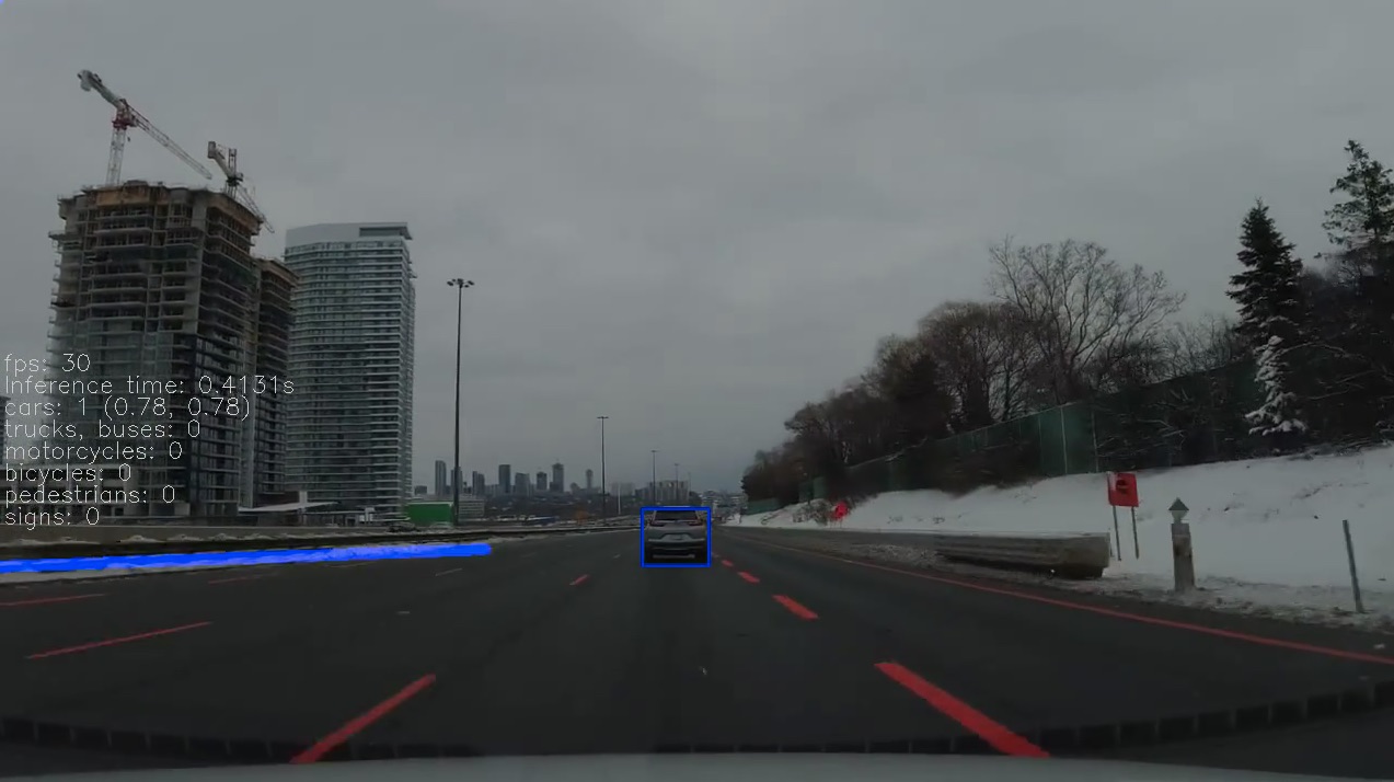
But there are more scenarios we did not tune the model for. In figure 4, the lane colour is different. As you can see, the model fails to output a proper line, and instead outputs a line to the left. What happened here is most likely that it found something like a lane line pointing to the left and extrapolated to the end of the frame.

In figure 5 you can see the cases so far in more detail in the short video.
Figure 5: Lane line detection in three different scenarios.
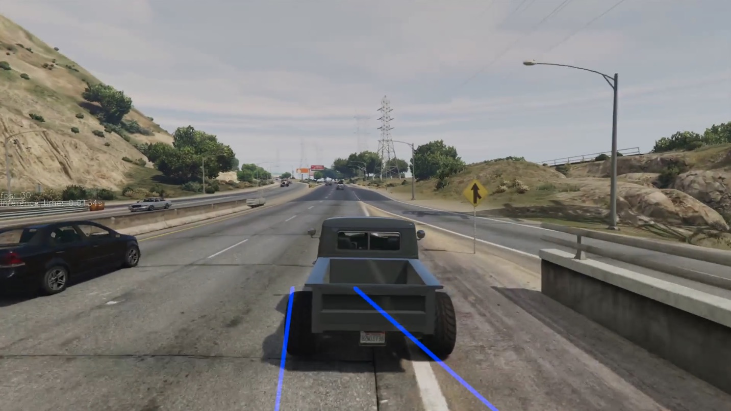
In the examples so far, the parameter that changed was the road itself. However, there are more parameters which influence the distribution. For instance, in figure 6 you can see what happens if both the road changes and the frames are from the video game GTA Online instead of the camera from earlier.
Despite the lanes being geometrically similar since both are on North American freeways the pipeline fails completely to detect them. One reason is that because of the camera angle, which shows the truck, the lanes do not fall into the region of interest which was defined earlier based on frames such as in figure 2. The result is that either no lane lines are detected, or arbitrary ones which do not align with the actual road markings which you can see in the video in figure 7.

Figure 7: The lane line detection pipeline completely fails on the data from GTA Online, because the camera angles are very different. This causes the lanes to fall outside of the region of interest which hides the lines from the detector part.
Conclusion
In conclusion, before heading into a ConvNet-based solution which requires a lot of labels and hardware-intensive training, it can be beneficial to consider how much variation there is in the problem at hand. If the domain is relatively static, a non-learning approach might be a cheaper and faster solution. We have seen this in the example of lane line detection based on a simple pipeline and tuned for a straight freeway. As long as the domain does not change, this simple pipeline delivers good results. However, it is more difficult to take into account variations such as different road surfaces, lane colours, curves, weather conditions etc. If we expect a lot of variation in the data a ConvNet could be better suited for the task.
If you are curious how lane detection with a ConvNet looks like, here is a link to a lane line detection model from NVIDIA’s Drive Lab.
