Mono vision distance approximation

When driving a car, it is not enough to know where other cars, pedestrians, and other obstacles are; it is also important to know how far these objects are away. For example, we may need to know if our distance to the vehicle in front of us is large enough for safe driving or to maintain a certain distance for adaptive cruise control. In driverless systems, this problem is often solved using radar or lidar. Alternatively, a stereo camera can be used for a vision-based solution. But what if there is only one camera available?

Here, we can use some geometry to our advantage. Generally, when using one camera, distances to objects of known width can be estimated using the perceived focal length of the camera. The focal length can be thought of as a magnification property of the camera lens. In figure 1, you can see the relations between width \(w\) and distance \(d\) in the physical space, and how both are perceived in the pixel space.

Figure 1: Physical dimensions on the top, and dimensions in the pixel space on the bottom.

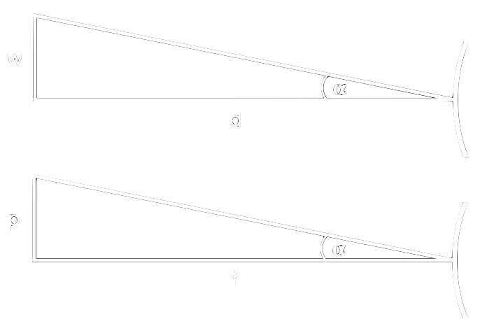
By expressing both using the angle \(\alpha\) we get:

\begin{equation} \tag{1.1} \tan(\alpha) = \frac{w}{d} = \frac{p}{f} \end{equation}

where \(w\) and \(d\) are in metres, and perceived distance \(p\) as well as perceived focal length \(f\) in pixels. Since \(\alpha\) is in both equations we can do

\begin{equation} \tag{1.2} \frac{w}{d} = \frac{p}{f} <=> f = \frac{p d}{w} <=> d = \frac{w f}{p} \end{equation}

which allows us to determine the perceived focal length from known object width and distance, as well as the physical distance to an object when focal length and object width are known.

For more details on this approach see this excellent post.

So let’s say we want to estimate the distance from the camera to a nearby vehicle. If we know the perceived focal length \(f\) in pixels of your camera we can use equation 1.2 to approximate distances in the wild. To do so, we assume that vehicles are 2m wide, which is the \(w\). Then we use for example an object detector to output a bounding box around it. This gives us the perceived width \(p\) in equation 1.2, with which we get the distance \(d\).

Implementation

Now that we know the basic idea let’s see how this can be implemented. For the following I assume the perceived focal length of the camera is already known.

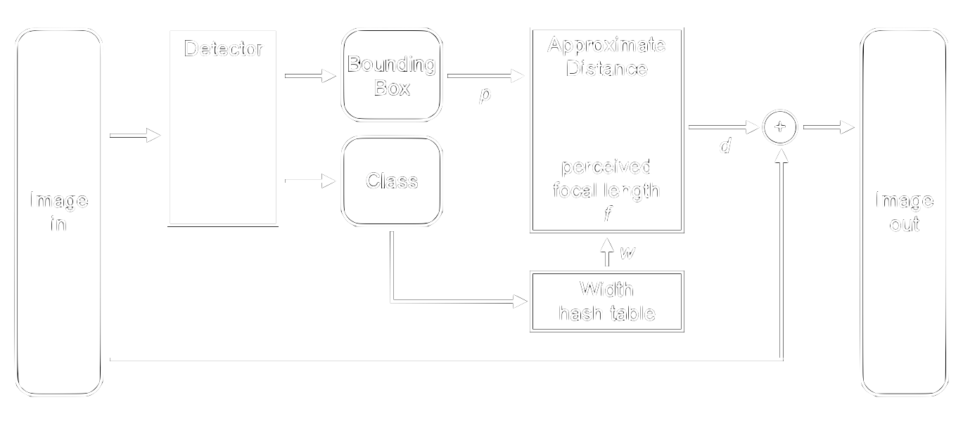
Given \(f\) we base our approximation on the width \(w\) of the object. We can store known widths for object classes in a hash table to quickly look them up. Our object detector gives us both the perceived width \(p\) in form of the bounding box width, as well as the object class. We then use this outputed class to look up the object width and calculate the approximated distance using equation 1.2. Figure 2 shows this architecture.

Figure 2: Distance approximation architecture

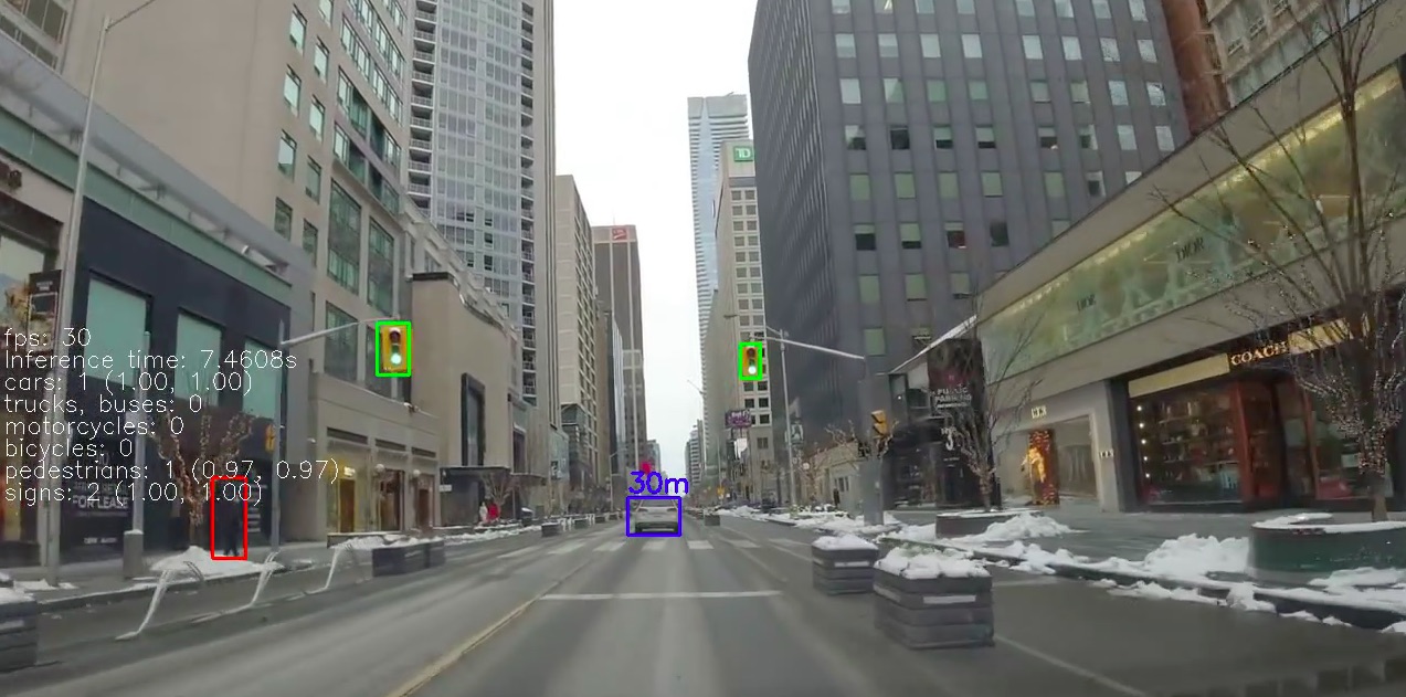
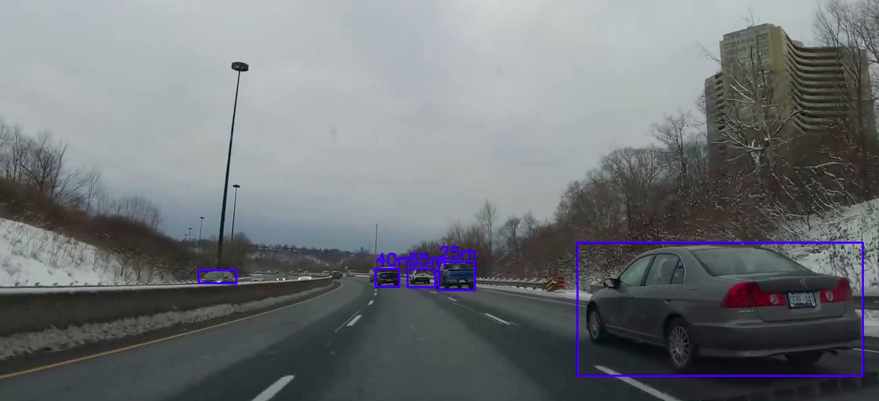
In figure 3 you can see an example output for the vehicle class.

Figure 3: Distance approximation to vehicle seen from the rear.

This approach works well as long as we don’t violate our assumption of known object width. Hence, this approach performs poorly when a vehicle is viewed from the side as opposed to from the rear. In figure 4 we see such a case. Here, the width of the bounding box around the vehicle represents a length greater than 2m, which leads to an error proportional to the width.

Figure 4: Viewing the vehicle form the side invalidades the vehicle width assumption.

To mitigate this problem, in the approximation, we introduce two measures. First, we observe that when we look at a vehicle from the rear first and then from the side that the bounding box’s width grows, but the height remains constant. Thus, we can define a height-to-width ratio and threshold against it. If this ratio falls below a threshold we assume that we are looking at the vehicle from the side and don’t output a distance, or provide a different \(w\) in the hash table for this view.

Figure 5: Vehicle moving into view from the side causes valid aspect ratios for the bounding box since the vehicle is partially occluded.

With this approach we still have an edge case. In figure 5, you can see a vehicle entering the image on the left. The detector highlights it correctly with a bounding box. However, since it is only partially visible, the height-to-width threshold does not filter out this case. To make sure that we only consider fully visible vehicles, we define a region of interest in which we want to apply the distance approximator only. Specifically for the vehicle example, we filter out \(\frac{1}{4}\) on each side of the image.

Finally to compensate for errors which result from the aforementioned simplifications, we round the approximated distances to the nearest 5m.

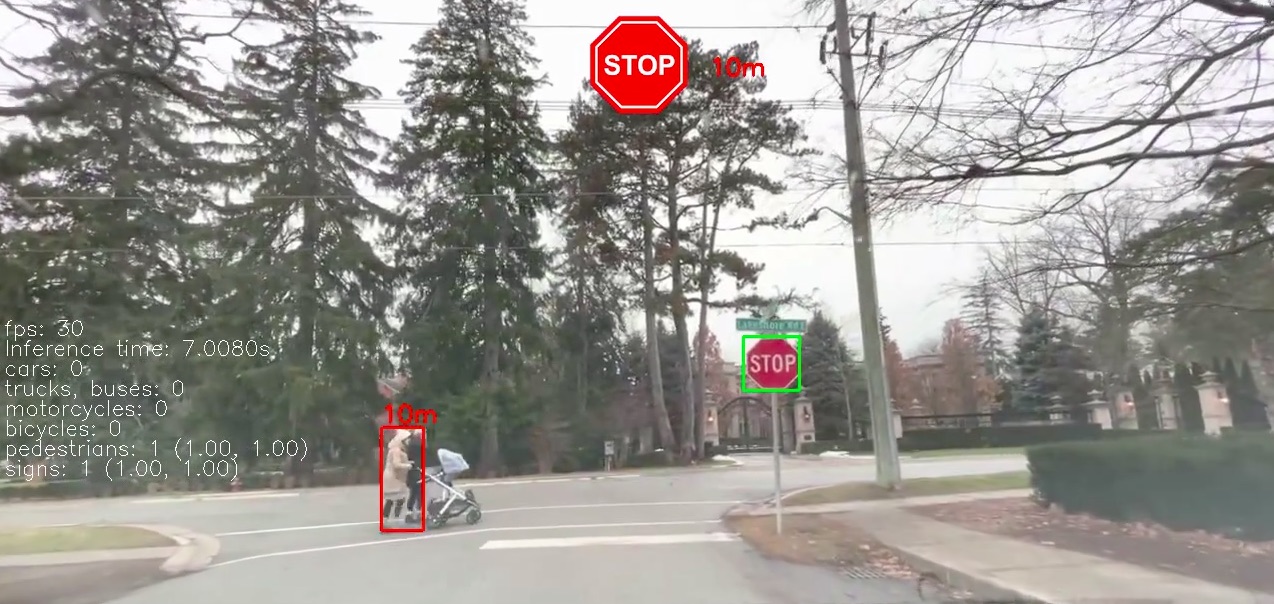
By introducing this height-to-width ratio threshold we have made the assumption that objects are always longer than they are wide, and that the length varies. Two examples for classes where there is less such variation are pedestrians (width exceptions due to poses) and stop signs. Figure 6 shows an example of both. The stop sign seems to be a simple case since there are only a few sizes allowed, and they are mostly mounted at similar height. But at the same time, they are on the side of the road so we have to be careful with our region of interest. The bottom line is that we have to look at the threshold and the region of interest separately for each class.

Figure 6: Stop signs can be detected well with the described approach due to their defined sizes.

Limitations

Since we had to make some assumptions for our rule-based system we should ask what price we paid.

Firstly, the whole system is based on the perceived focal length and the assumed width of the object. Since we match the bounding box width with the assumed width, the performance also depends on how well the predicted bounding box matches the ground truth box (often quantified by the mAP, see here for details), and how consistent this is over subsequent frames. You can see the effect of inconsistent sizes in the video below, where occasionally the predicted distance alternates between two values in subsequent frames.

Figure 7: Distance approximation depends linearly on defined width, and detected bounding box. Note how the numbers might alternate due to inconsistent bounding box widths in subsequent frames.

Secondly, we rely on the object detection model to provide us the correct class, so that we can look up the correct object width and apply the correct threshold to the height-to-width ratio. We have observed some misclassifications of traffic cones as vehicles for example which results in false calculated distances.

How to improve

So we had an idea for how to estimate distances based on a single camera output and described the system’s obvious limitations. And overall it works quite well as you can see in the video below.

Figure 8: Using the described system to approximate distances to vehicles, pedestrians and stop signs in different scenarios.

But this system can be improved. Generally, we can look at our system from two sides: a learned part which provides us the perceived dimension, and a rule-based part which provides the physical object width and puts everything together.

The first potential improvement focuses on the rule-based part. Here we could include depth information to resolve inconsistencies in calculating the distances of multiple objects. For example, when we have a stop sign and know that a person is walking behind it, we should output \(d_{person} > d_{sign}\). This depth information could come from a different network which is trained to perform monocular depth estimation.

A second idea tries to improve the rule-based part by providing more assumed widths for an object. For example, we could add an assumed width for a view from the side \(w_{side}\) in addition to the rear \(w_{rear}\). If the height-to-width ratio is smaller than a certain threshold \(a_{thresh,rear}\), but greater than \(a_{thresh,side}\) then we retrieve \(w_{rear}\), but if it it also smaller than the side threshold we take \(w_{side}\).

Alternatively, we could train the model with angle labels in addition to the class labels. Then the model would give us a bounding box, class and viewing angle which we could then use to look up more accurate assumed distances. By moving the viewing angle detection into the learned part we would avoid thresholding multiple times. But why stop there?

If we have data with distance labels we can move the whole rule-based part into the learned part. We would end up with one convnet which we could train end to end. This is exactly what NVIDIA did.

I wish I had NVIDIA’s data available. In the meantime we have seen that with a little creativity you can get decent results as well.