How to use COCO for Object Detection

To train a detection model, we need images, labels and bounding box annotations. The COCO (Common Objects in Context) dataset is a popular choice and benchmark since it covers a variety of different objects in different settings. Here you can learn more about how models are evaluated on COCO.

Here is my video version of this post:

Setting up

To get started, we first download images and annotations from the COCO website. We create a folder for the dataset and add two folders named images and annotations. Next, we add the downloaded folder train2017 (around 20GB) to images and the file instances_train2017.json to annotations. Our dataset folder should then look like this:

cocoDataset/
├── annotations/
│   ├── instances_train2017.json
├── images/
│   ├── train2017/
│       ├── 000000000009.jpg
│       ├── ...

Images - Images are in the .jpg format, of different sizes and named with a number. All image names are 12 digits long with leading 0s.

COCO annotation file - The file instances_train2017 contains the annotations. These include the COCO class label, bounding box coordinates, and coordinates for the segmentation mask. Next, we explore how this file is structured in more detail.

Annotation file structure

The annotation file consists of nested key-value pairs. On the top level there are five such objects:

'info'
'licenses'
'categories'
'images'
'annotations'

In Python we can access these objects by loading the file with the json module.

import json
path = "./annotations/instances_train2017.json"
f = open(path)
anns = json.load(f)
print(anns.keys())
 
>> dict_keys(['info', 'licenses', 'images', 'annotations', 'categories'])

The first two objects contain information regarding the dataset such as date of creation etc. and the licenses under which the images are used. For example, the first license is

{'url': 'http://creativecommons.org/licenses/by-nc-sa/2.0/',
  'id': 1,
  'name': 'Attribution-NonCommercial-ShareAlike License'}

Before we explore the remaining objects let’s define three variables.

category_id	- Maps a label to the class name
image_id	- Image name without file extension and leading zeros
annotation_id	- Annotation identifier

Each of these ids is unique.

The categories key contains a list of category objects. These map the category_id to the classname. For example, the first two are

{'supercategory': 'person', 'id': 1, 'name': 'person'},
 {'supercategory': 'vehicle', 'id': 2, 'name': 'bicycle'}

The image object contains image meta information.

{'license': 4,
  'file_name': '000000522418.jpg',
  'coco_url': 'http://images.cocodataset.org/train2017/000000522418.jpg',
  'height': 480,
  'width': 640,
  'date_captured': '2013-11-14 11:38:44',
  'flickr_url': 'http://farm1.staticflickr.com/1/127244861_ab0c0381e7_z.jpg',
  'id': 522418}

Note the two fields file_name and id (which is the image_id) are the same except the leading zeros in the file name (and the extension). That means we can use the image_id to later retrieve image files.

For each image, there are one or multiple annotation objects. Each one of these annotations contains multiple key-value pairs

{'segmentation': [[239.97,
   260.24,
...   
222.04,
   228.87,
   271.34]],
 'area': 2765.1486500000005,
 'iscrowd': 0,
 'image_id': 558840,
 'bbox': [199.84, 200.46, 77.71, 70.88],
 'category_id': 58,
 'id': 156}

The image_id maps this annotation to the image object, while the category_id provides the class information. Each annotation is uniquely identifiable by its id (annotation_id).

The bounding box field provides the bounding box coordinates in the COCO format x,y,w,h where (x,y) are the coordinates of the top left corner of the box and (w,h) the width and height of the box.

COCO api

If you don’t want to write your own code to access the annotations you can get the COCO api.

As a brief example let’s say we want to train a bicycle detector. To get annotated bicycle images we can subsample the COCO dataset for the bicycle class (coco label 2).

First, we clone the repository and add the folders images and annotations to the root of the repository. Then we can use the COCO api to get a list of all image_ids which contain annotated bicycles.

from pycocotools.coco import COCO

ann_file = “../annotations/instances_train2017.json”
coco=COCO(ann_file)
 
# Get list of category_ids, here [2] for bicycle
category_ids = coco.getCatIds(['bicycle'])
>> [2]

# Get list of image_ids which contain bicycles
image_ids = coco.getImgIds(catIds=[2])
print(image_ids[0:5])
>> [196610, 344067, 155652, 417797, 294918]

With this list of image_ids we can get annotations. For example, to get all annotations containing bicycles in the image 000000196610.jpg we use two filters, which results in five bicycle annotations.

# Get all bicycle annotations for image 000000196610.jpg
annotation_ids = coco.getAnnIds(imgIds=196610, catIds=[2])
print(len(annotation_ids))
>> 5

These five annotation objects can then be loaded into a list anns

anns = coco.loadAnns(annotation_ids)

Now we can access the bounding box coordinates by iterating over the annotations.

for ann in anns:
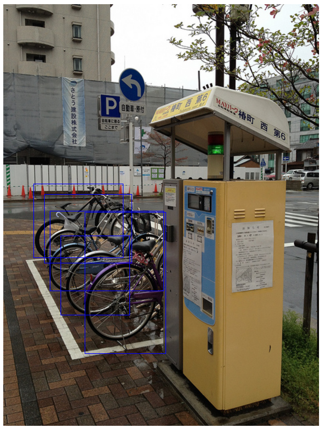
    print(ann['bbox'])

To visualize the image with all bicycle annotations we can use matplotlib and PIL for example.

from PIL import Image
import matplotlib.pyplot as plt
import matplotlib.patches as patches
 
image_id = 196610
 
images_path = "./images/train2017/"
image_name = str(image_id).zfill(12)+".jpg" # Image names are 12 characters long
image = Image.open(images_path+image_name)
 
fig, ax = plt.subplots()
 
# Draw boxes and add label to each box
for ann in anns:
    box = ann['bbox']
    bb = patches.Rectangle((box[0],box[1]), box[2],box[3], linewidth=2, edgecolor="blue", facecolor="none")
    ax.add_patch(bb)
 
ax.imshow(image)
plt.show()

Figure 1 shows the image with the drawn bounding boxes.

Figure 1: Example for COCO bicycle annotations.

And that is how we can access the bicycle images and their annotations.

In conclusion, we have seen how the images and annotation of the popular COCO dataset can be used for new projects, particularly in object detection.