Deconvolutions and what to do about artifacts

Figure 1: Example for checkerboard patterns on image generated by a network with deconvolutions.

Introduction

Convolutional neural networks are an efficient way to extract features from images by convolving inputs with learned filters. While this operation typically reduces the spatial resolution of the input, the reverse operation can be used to increase the spatial resolution, thus performing upsampling tasks. This is called a deconvolution, transposed convolution, or fractionally strided convolution, depending on the parameters used.

Common applications of deconvolutions include semantic segmentation Long et al. (2015), super-resolution Shi et al. (2016), and other image generating tasks such as real-time style transfer Johnson et al. (2016).

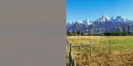
However, when networks generate images from lower resolutions using deconvolutions, the resulting images often have checkerboard artifacts, see for example figure 1. Odena et al.(2016) provides an excellent discussion about the reasons for this.

This post reviews what deconvolutions are, why they tend to produce artifacts, and what to do about it based on Odeana et al. Then we dive deeper into these findings with experiments. To follow along, you can get the code here.

What deconvolutions are

Deconvolutions were first introduced by Zeiler et al.(2010) for unsupervised learning of features, and then later used to visualize the learned features of a convnet in Zeiler et al. (2013).

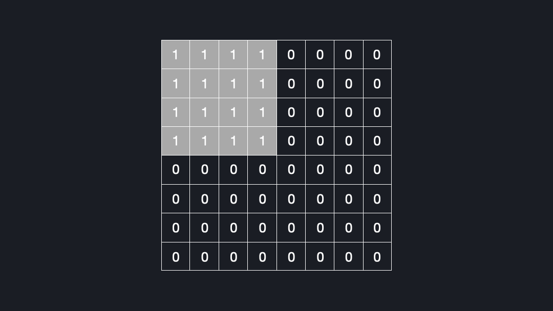
To understand deconvolutions we need to know that we can express (direct) convolutions in a flattened matrix. If you want to learn more about convolutions, kernels, and strides see our post about convnet basics. Figure 2 shows how an input of size $4x4$ is convolved with a kernel of size $3x3$ and stride $1$ to generate an output of size $2x2$. Here, the kernel has four positions in which the weights are multiplied with the corresponding cells of the input.

In the corresponding matrix, each row contains the outputs from a kernel position. For each position the output is flattened, yielding $0s$ where the kernel does not cover an input cell. To compute the output, one can multiply the input with this matrix \(C\), as a sanity check of the dimensions (4x16) x (16 x num_filters) = (4 x num_filters) confirms.

In the backward pass during training we want to “undo” the convolutional operation to propagate the loss through the network, meaning we want to go from shape $2x2$ to $4x4$. This can be achieved by transposing the matrix \(C\). Transposing the matrix is a linear operation and fully reversible. Note that this means that the kernel defines both the forward and backward operation. Interestingly, this is exactly what we want for a deconvolution. That is why the deconvolution is also called a transposed convolution [Dumoulin et al. (2018)].

Figure 2: Direct convolution expressed in a matrix C by flattening the input and the kernel. By transposing the matrix one can undo the convolution, leading to a transposed convolution. Adapted from Dumoulin et al. (2018).

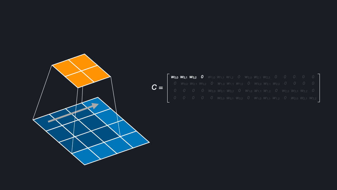
Figure 3 on the left shows an alternative way to increase the spatial resolution from $2x2$ to $4x4$. We can upsample the input to the shape $6x6$, and then apply a direct convolution with kernel size of $3x3$, stride $1$, see figure 2 left. This is an example that every deconvolution can also be implemented with upsampling in some way followed by a convolution. One downside is that upsampling followed by a convolution is computationally inefficient for small feature maps. In this example, only $4$ out of $36$ cells contain the original information.

Figure 3: Deconvolutions and why they are also called fractionally-strided convolutions depending on the padding and strides. Left: to get an output (top) of shape 4x4 from an input of shape 2x2 (bottom, blue) the input can be upsampled to 6x6 and then convolved with stride 1. This is equivalent to a transposed convolution from input 2x2 to output 4x4. Right: For some combinations of input/output/stride padding between elements is required, which leads to fractional strides. Adapted from Dumoulin et al. (2018).

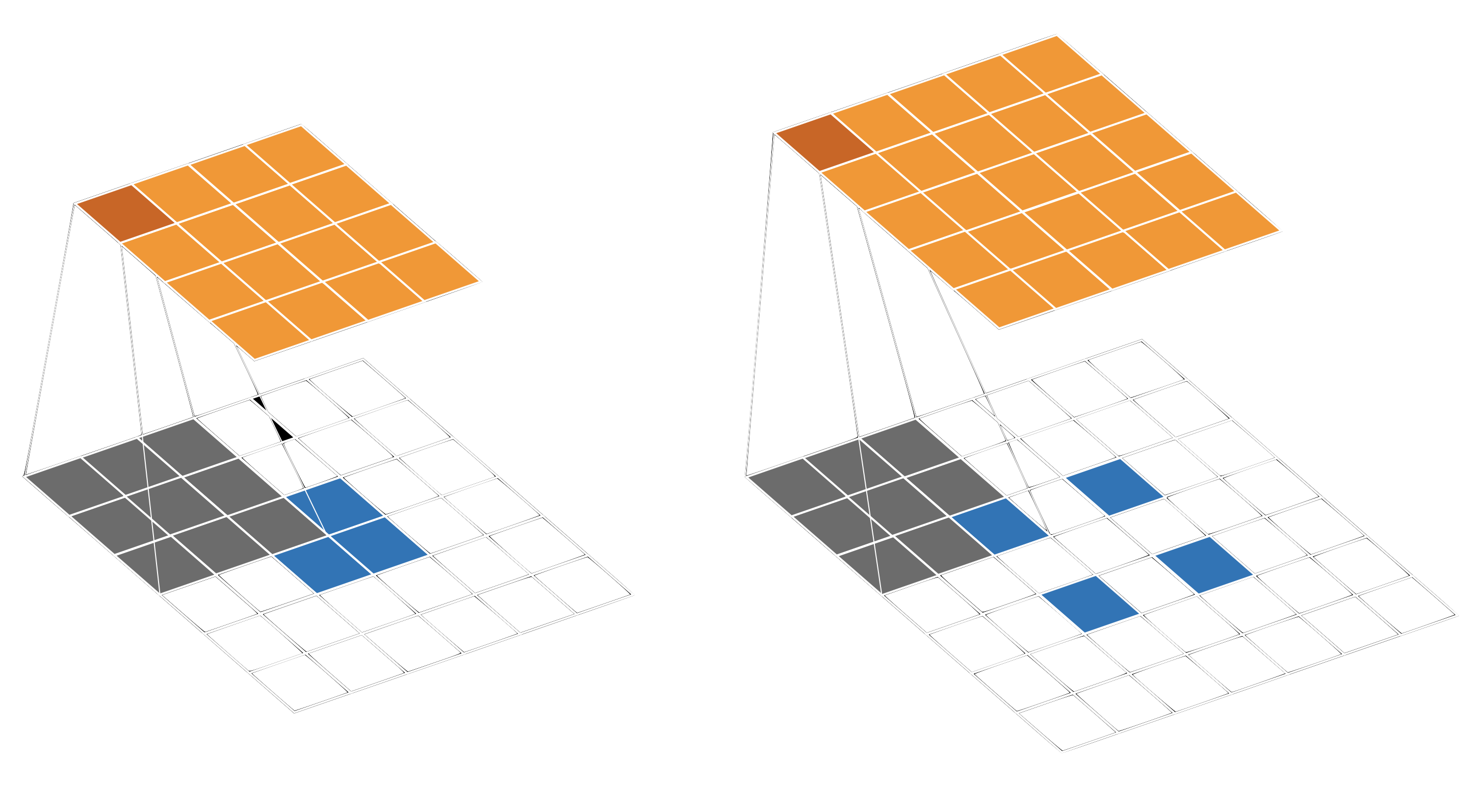
Depending on the shape of the input and output, we can also pad between input elements, see right side of figure 3. Here, an input of shape $2x2$ leads to an output of shape $5x5$, with a kernel size of $3x3$ and a stride of $1$. Because of the spacing between the elements, the kernel now has to move two positions to cover two cells which were neighbours before the padding, instead of one. Hence, this particular stride is also called $\frac{1}{2}$, or fractionally. That is why a deconvolution (with padding between the input elements) is also called a fractionally strided convolution [Dumoulin et al. (2018)].

Why deconvolutions lead to artifacts

Now that we know what deconvolutions are, let’s see why they can lead to checkerboard artifacts. Let’s assume we convolve a kernel size of $3x3$ with an input using a stride of $2x2$. Figure 4 shows how many times each cell is seen by the kernel.

Figure 4: Overlap leads to checkerboard patterns.

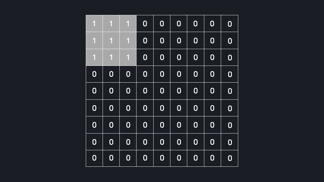
As you can see, some elements are visited up to four times, while others are just once. This is the reason for the checkerboard artifacts!

Figure 5 shows that these artifacts are a network-inherent issue and not related to training. Already after the first epoch you can spot the artifacts, and they remain largely unaffected by training. This was already pointed out for GANs by Odean et al. (2018).

Figure 5: Artifacts are model-inherent and not related to training. Left: Image after the first iteration. Right: After 70,000 iterations (10 epochs), the artifacts have not changed much.

How to avoid checkerboard artifacts

Odean et al. (2018) describe three ways to limit the effects.

First, one can use a deconvolution with a large filter and a stride of $1$ as the last layer. This seems to smooth out artifacts and is used by many models. In my own experiments this does not help sufficiently.

The second approach is to choose a kernel size that is divisible by the stride. For example, if a kernel of shape $4x4$ is used, a stride of 2 reduces the artifacts, see figure 6. Like in the example of figure 4, the maximum number of times a cell is marked by the kernel is 4. However, these cells are all adjacent in the centre, largely reducing the checkerboard artifacts.

Figure 6: If the stride (here 2) divides the kernel size (here 4x4) the effect of artifacts due to overlap is reduced since there aren't any gaps between the most frequently marked cells. The numbers indicate how many times a cell is marked by the kernel.

To fully avoid artifacts, it is best to avoid the deconvolution and implement a padding/upsampling directly followed by a convolutional layer instead. As discussed above, this is equivalent to a deconvolution, albeit less computationally efficient due to the additional upsampling operation.

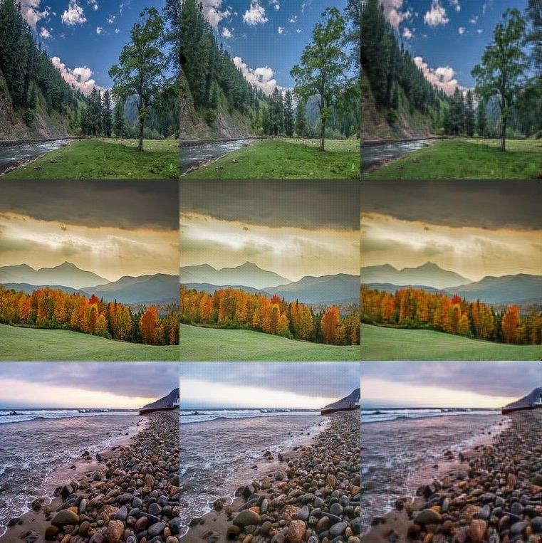
Figure 7 shows how the results of a model change. On the left you can see 3 images. In the centre the images show reconstructions with a model which has deconvolutions. On the right you can see the same model where the deconvolutions have been substituted with upsampling followed by a convolutional layer. The two models are the transformation networks trained with a pixel loss for 10 epochs on around 7,000 images from the kaggle art dataset.

Figure 7: Images reconstructed by a model with deconvolutions (centre) and one with substituted deconvolutions (right). Originals are on the left.

Conclusion

There are many names for deconvolutions, but they all lead to the same result which can also be implemented with a direct convolution and padding/upsampling of the input. To avoid checkerboard artifacts, which typically occur on images generated by models which use deconvolutions to increase the spatial resolution, it is best to avoid these deconvolutions entirely and use their slightly less efficient equivalents of convolutions on upsampled inputs.

References

Long, Jonathan, Evan Shelhamer, and Trevor Darrell. “Fully Convolutional Networks for Semantic Segmentation.” ArXiv:1411.4038 [Cs], March 8, 2015. http://arxiv.org/abs/1411.4038.

Shi, Wenzhe, Jose Caballero, Ferenc Huszar, Johannes Totz, Andrew P. Aitken, Rob Bishop, Daniel Rueckert, and Zehan Wang. “Real-Time Single Image and Video Super-Resolution Using an Efficient Sub-Pixel Convolutional Neural Network.” In 2016 IEEE Conference on Computer Vision and Pattern Recognition (CVPR), 1874–83. Las Vegas, NV, USA: IEEE, 2016. https://doi.org/10.1109/CVPR.2016.207.

Johnson, Justin, Alexandre Alahi, and Li Fei-Fei. “Perceptual Losses for Real-Time Style Transfer and Super-Resolution.” ArXiv:1603.08155 [Cs], March 26, 2016. http://arxiv.org/abs/1603.08155.

Odena, et al., “Deconvolution and Checkerboard Artifacts”, Distill, 2016. http://doi.org/10.23915/distill.00003.

Zeiler, Matthew D., Dilip Krishnan, Graham W. Taylor, and Rob Fergus. “Deconvolutional Networks.” In 2010 IEEE Computer Society Conference on Computer Vision and Pattern Recognition, 2528–35. San Francisco, CA, USA: IEEE, 2010. https://doi.org/10.1109/CVPR.2010.5539957.

Zeiler, Matthew D., and Rob Fergus. “Visualizing and Understanding Convolutional Networks.” ArXiv:1311.2901 [Cs], November 28, 2013. http://arxiv.org/abs/1311.2901.

Dumoulin, Vincent, and Francesco Visin. “A Guide to Convolution Arithmetic for Deep Learning.” ArXiv:1603.07285 [Cs, Stat], January 11, 2018. http://arxiv.org/abs/1603.07285.