ConvNet Basics
Extracting features from a grid of pixel intensities is very difficult considering that there is so much variance in object shape, perspective, lighting, colour, amongst other things. Algorithms such as Scale Invariant Features Transforms or Histograms of Oriented Gradients can do that fairly well, but they have to be tailored to extract features from images. A fully connected neural network could be used to avoid such manual tuning, though likely at great computational costs. To illustrate this cost, a 1080p colour image (\(1920x1080x3\) values) fully connected to a layer with just \(100\) neurons would have \(622,080,000\) connections. The computational cost for that many connections would be huge and would scale with the number of pixels multiplied by the number of neurons in the first layer. Additionally, the amount of memory required just to store the weights of the model would be huge.
A pixel in the top left corner of the image is unlikely to have much relation to one in the bottom right, so extracting features should look at the relationship of pixels with its neighbours. Convolutional layers detect features by finding relationships about a pixel and its neighbours using learnable weights. These features can then be combined together using further convolutions to make more complex features until they are fed into a classifier to create the output.
Convolutional layers work similarly to the edge and corner detectors used in SIFT and HOG; however, convolutional neural networks learn the weights used in the Kernel from the data rather than using empirical values. These learned weights can therefore be used to detect features unique to the dataset. The following section will go into further depths on how these convolutions work.
How Convolutional Layers Work
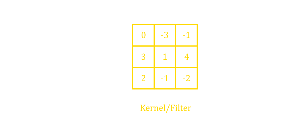
A convolutional layer works by completing element-wise multiplications between the layer’s kernel and the input (figure 10). A kernel is simply a grid of trainable weights that are convolved across the image. Figure 11 shows the kernel on top of the top left section of the input to illustrate a convolution. Element-wise multiplications are performed between the kernel and the parts where the kernel overlaps with the image. Then, the resultant grid of numbers (figure 11 top) is summed up together to create a single entry in the output feature layer. The kernel then slides across the input rightwards and downwards and the previous operations are repeated to create all of the other entries in the output. Sliding the kernel around and performing the same operation permits the same features to be detected when an object is translated vertically or horizontally.

A convolutional layer creates features by looking at a pixel and its neighbours, giving each pixel in that area a weight, and summing them up to create a grid of features or a feature map. For example, figure 12 shows a convolutional kernel that can detect vertical lines. In this figure, the input has a vertical boundary right in the middle separating the 0’s and 10’s. The kernel used only activates when the numbers on the left are greater than the numbers on the right, thus detecting vertical boundaries. As shown in the figure, it creates values of \(10\) separating the left and right side for the output, thus locating the vertical edge from the input. The same kernel rotated \(90°\) would give a horizontal line detector.
The vertical line feature detected in figure 12 is a rather simple feature. By using many different kernels, many different features may be detected. The next layer may then combine those features to detect more and more complex features such as boxes, circles, wheels, and then eventually even faces in much deeper layers. All of the kernels use trainable weights, adapting the detected features based on the training dataset.
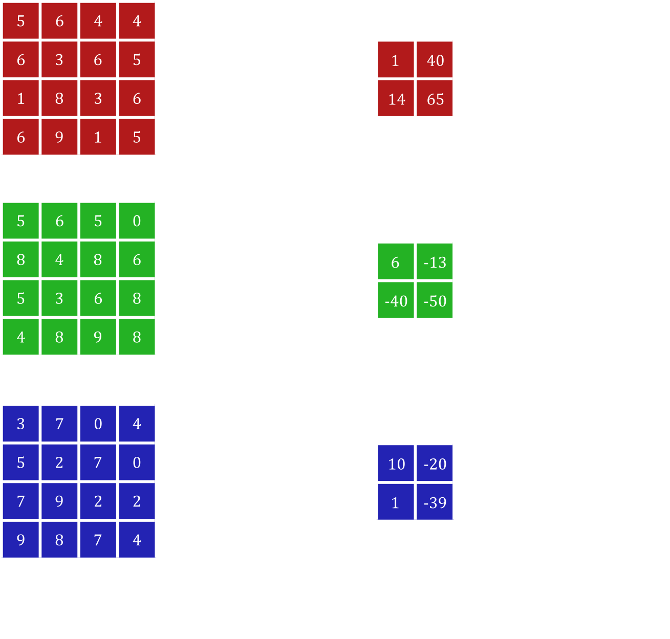
All of the convolutional layers so far have only processed inputs with only two dimensions. For 3-dimensional inputs such as colour images with \(3\) colour channels, the kernel is also 3-dimensional to find relationships between colour channels. The outputs of these convolutions are also 3-dimensional when using more than one kernel. Figure 13 shows how convolutional layers deal with inputs with multiple channels, where the convolution acts on each channel individually with different weights before summing them up. In this way, even a \(1x1\) convolution may be useful in finding relationships between the different features in the same space.
Padding
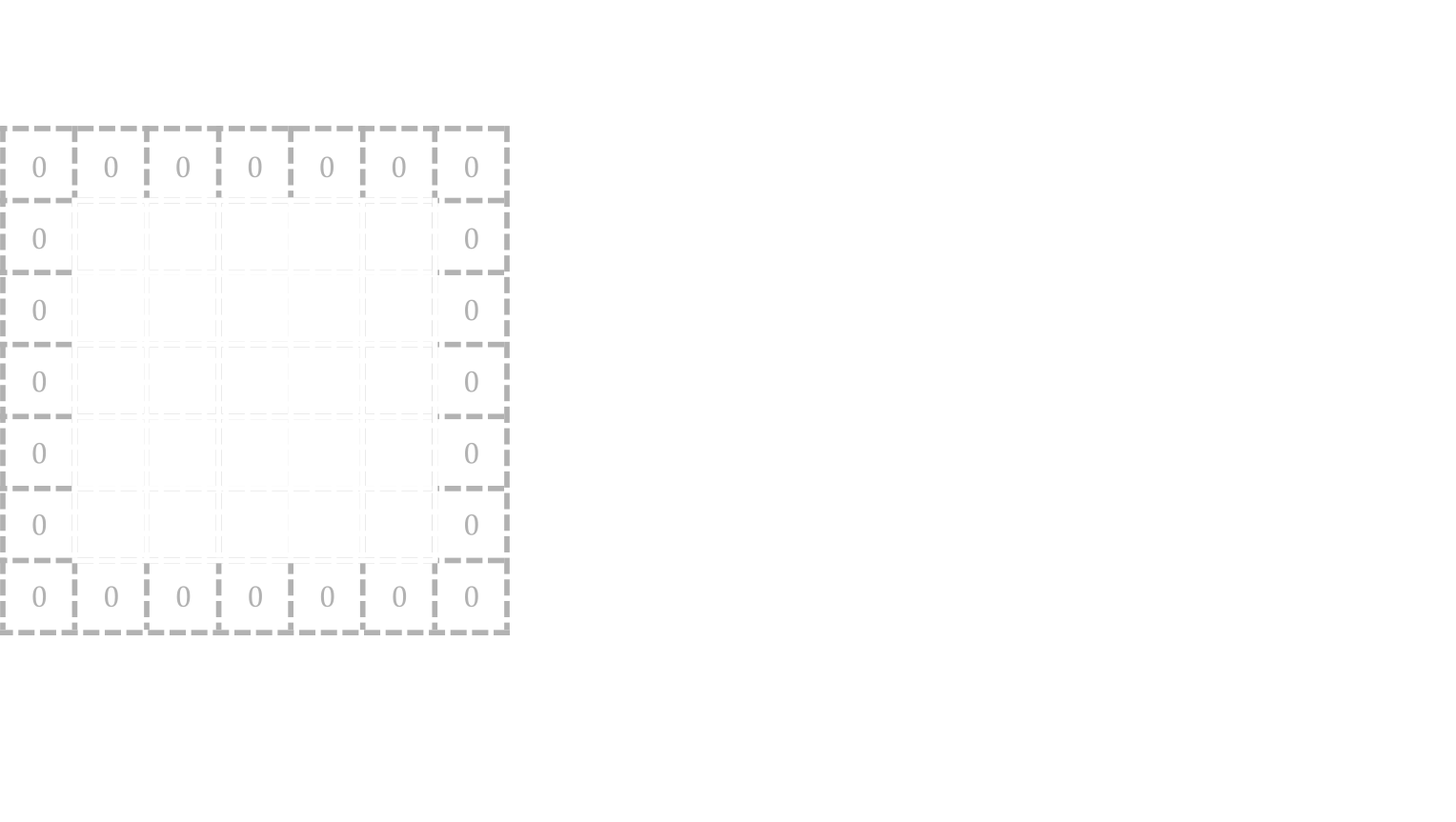
In all of the figures above, the outputs have shrunk compared to the inputs. This is because there are fewer spaces available around the edges and corners of the images that can fit the kernel. After a couple of dozen or hundreds of convolutions, the image would have shrunk far too much and information around the edges and corners of the original image would be lost. There is, however, a simple solution to this problem: padding the borders of the input with zeros or more simply zero padding
Figure 14 shows the difference between completing a convolution with and without padding. With padding, the convolved features maintain the original resolution \((5x5)\) of the input; whereas, without padding, the output shape shrinks to be a \(3x3\) grid. Notably, without padding, the corners of the input are only involved in \(1\) value in the output rather than the \(9\) at the centre, deemphasizing the feature information around the edges of the input. One can imagine that feature information can be lost around the edges of the input image without the use of padding, especially after several convolutional layers.
Pooling Layers
Up to now, convolutions are able to extract features, but not able to substantially shrink large images into more manageable sizes. One option is to increase how many pixels to slide the kernel over during the convolution calculations, also known as the stride, to reduce the size of the output. However, this may overlook some key features from skipping these key values. The use of pooling layers helps avoid this loss of feature information while still being able to reduce the resolution of the feature map.
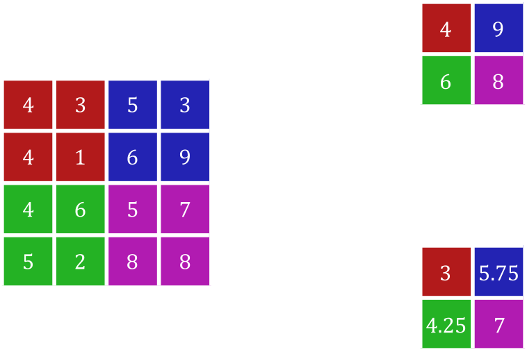
Figure 15 shows the use of two different pooling operations using a stride of \(2\). In a way, it works similar to a convolution except that instead of multiplying each element with weights, it returns the maximum (max pooling) or average (average pooling) value. Even the size of the ‘kernel’ and stride can be defined similarly. However, two notable differences are that this operation involves no trainable weights and that normally the output is a fraction of the original size.
An Example Architecture
Now that you are familiar with convolutional layers, pooling layers, and padding, it might be helpful to see an example of a full convolutional neural network to see how they can be used together.
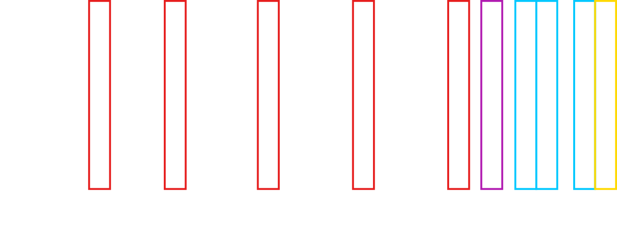
Figure 16 shows the architecture of VGG-16 [18], a neural network that competed in ImageNet Challenge 2014 and won second place in the image classification challenge. Its most notable improvement over its predecessor, AlexNet, was the use of multiple \(3x3\) convolutional layers rather than using larger \(7x7\) or \(5x5\) convolutional layers.
VGG-16 shows a typical convolutional neural network architecture. As can be seen in figure 16, it alternates between using a couple convolutional layers and a max pooling layer which lowers the resolution of the features (e.g. \(224x224\) to \(112x112\)). The result is then flattened and fed into a handful of fully connected layers before being outputted using a softmax function. Additionally, this neural network uses the same padding for all of its convolutional layers which is fairly commonly used for convolutional neural networks. Notably, as you go deeper into the neural network, while the resolution goes down, and the number of channels progressively goes up (e.g. \(224x224x64\) to \(112x112x128\)).
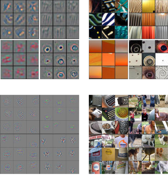
The idea of using neural networks is to build simple functions and then combining them together to form more and more complex functions in the deeper layers. Similarly for convolutional layers, the early layers are used to detect very simple features that combine together in the deeper layers to form larger and more complex features. Figure 17 shows reconstructed patterns that cause high activations in a feature map in a convolutional neural network [19]. It demonstrates that the earlier layer (layer 2) detects colours and shapes while the deeper layer (layer 5) detects patterns of dots, faces, and words. This supports the theory that convolutional layers may be able extract meaningful features rather than seemingly random relationships; though, there are the existence of adversarial examples which are inputs that can easily mislead a machine learning model. An entire section of this website is dedicated to adversarial examples.
Summary
- Convolutional layers can extract features by looking at each pixel with its neighbours and multiplying them element-wise with trainable weights and then summing them up
- Because the same operations are used throughout the image, convolutional layers can detect things that are translationally similar
- Padding is often used around the edges of an input to ensure that the output remains the same size
- Pooling layers are used to reduce the resolution of the input
- Oftentimes, convolutional neural networks will alternate between using convolutional and pooling layers
- Normally, deeper layers are smaller in resolution, but have larger numbers of channels
- Shallower layers tend to detect simple features while deeper ones detect more complex features
These convolutional neural networks provide the foundations for many of the more recent object classification, localization, and segmentation models such as R-CNN and YOLO which will be discussed in the next sections.
References
[19] Zeiler, M. D., & Fergus, R. (2013). Visualizing and Understanding Convolutional Networks. ArXiv:1311.2901 [Cs].http://arxiv.org/abs/1311.2901